4. Mathematical Representations
The objective of mathematical representations is to determine relationship among variables and develop mathematical model that reflects how the firm demand is affected by different variables.
Two analysis methods can be employed to discover the relationship – time series and regression analysis. Time series analysis is a simple measure of how dependent variable changes against the lapse of time. Time will be the only independent variable in the analysis. Regression analysis attempts to depict the relationships between independent and dependent variables so that dependent variable can be predicted. The relationship can be linear, exponential, power, polynomial, etc. There can one independent variable, as well as multiple variables.
In this project, our objective is to determine how
exogenous, endogenous, and firm specific variables combined affect the firm
demand.
1) Firm Demand (FD). The firm demand is calculated by the product of the total industry demand (TID) and the firm market share (MS).
= TID * MS
2) Total Industry Demand (TID). Total industry demand is expressed by the average firm demand (AFD) and the number of firms in the industry (N).
= AFD * N
Combine this formula with the formula in 1), the firm demand can be expressed
= AFD * N * MS
To simplify the formula, we create a new variable, called Normalized Market Share (NSOM) derived by N * MS. The final firm demand formula looks like this
=AFD * NSOM
3)
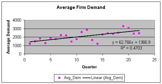
Average Firm Demand (AFD). To explore the use of regression modeling for
obtaining more reliable forecasts, scatter plot is a simple start point to
visualize if there are any patterns in the industry demand.

Figure
1 – Average Firm Demand Time Series
From the above scatter spot chart, we clearly see
a pattern that the average firm demand is in an upper-tick trend as time is
passing by. Time series analysis will be a perfect fit for forecasting the
future demand. By extending the trend we will have a fairly good estimate of AFD.
|
SUMMARY
OUTPUT |
|
|
|
|
|
|
|
|
|
|
|
|
|
|
|
Regression
Statistics |
|
|
|
|
|
|
|
Multiple
R |
0.685774645 |
|
|
|
|
|
|
R
Square |
0.470286863 |
|
|
|
|
|
|
Adjusted
R Square |
0.443801206 |
|
|
|
|
|
|
Standard
Error |
443.2454672 |
|
|
|
|
|
|
Observations |
22 |
|
|
|
|
|
|
|
|
|
|
|
|
|
|
ANOVA |
|
|
|
|
|
|
|
|
df |
SS |
MS |
F |
Significance
F |
|
|
Regression |
1 |
3488515.89 |
3488515.89 |
17.75628469 |
0.000426705 |
|
|
Residual |
20 |
3929330.883 |
196466.5442 |
|
|
|
|
Total |
21 |
7417846.773 |
|
|
|
|
|
|
|
|
|
|
|
|
|
|
Coefficients |
Standard
Error |
t
Stat |
P-value |
Lower
95% |
Upper
95% |
|
Intercept |
1366.87013 |
195.6341059 |
6.986870328 |
8.83431E-07 |
958.7847254 |
1774.955534 |
|
PRD |
62.76623377 |
14.89532626 |
4.213820676 |
0.000426705 |
31.69514209 |
93.83732545 |
Table 1 – Average Firm
Demand Time Series Result
AFD = 62.766 * T + 1366.9
(equation 1)
We could use Crystal Ball
Predictor 1.3 to perform time series analysis as well. Predictor actually
provides more accurate time forecast compared with linear regression analysis
because it can follow the seasonality embedded in the original data while linear
regression analysis tries to represent the trend by one straight line. The
detailed comparison between the two can be found in the file CB_Forecast_Avg_Dem.xls.
For the simplicity of our model, we adopted the result from the linear
regression analysis, which still gives us a fairly good estimate of the
relationship between the demand and time.
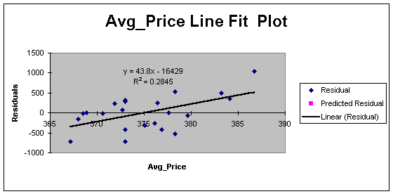
However, the time is not the only factor explaining the changes in the demand. This is testified by the fairly large residuals between historical data and predicted values by the analysis (See demand.xls). We have to introduce other factors, such as Average Price (Avg_Price), Average Advertising Expenditures (Avg_Adv), and Average R&D (Avg_RD), to analyze their influences on the residuals. Both Excel Regression Analysis function and SAS Stepwise procedure can help us find the relationship.
a. Regression Analysis by Using Excel
Using Excel to eliminate
variables that are not significantly related to the dependent variable can be
extremely cumbersome if lots of independent variables are involved to be tested.
We have to run regression analysis several times to obtain the final formula,
each time eliminating one variable with p-value greater than alpha. In our case,
we didn’t get the ideal result until regression analysis was run the 6th
time.
Residuals = -(43.8 * Avg_Price
– 16429) (equation 2)
|
SUMMARY OUTPUT |
|
|
|
|
|
|
|
|
|
|
|
|
|
|
|
|
|
Regression
Statistics |
|
|
|
|
|
||
|
Multiple R |
0.533422954 |
|
|
|
|
|
|
|
R Square |
0.284540048 |
|
|
|
|
|
|
|
Adjusted R Square |
0.248767051 |
|
|
|
|
|
|
|
Standard Error |
374.9185834 |
|
|
|
|
|
|
|
Observations |
22 |
|
|
|
|
|
|
|
|
|
|
|
|
|
|
|
|
ANOVA |
|
|
|
|
|
|
|
|
|
df |
SS |
MS |
F |
Significance
F |
|
|
|
Regression |
1 |
1118051.999 |
1118051.999 |
7.954045436 |
0.010571406 |
|
|
|
Residual |
20 |
2811278.884 |
140563.9442 |
|
|
|
|
|
Total |
21 |
3929330.883 |
|
|
|
|
|
|
|
|
|
|
|
|
|
|
|
|
Coefficients |
Standard
Error |
t
Stat |
P-value |
Lower
95% |
Upper
95% |
|
|
Intercept |
-16429.1921 |
5825.910028 |
-2.820021598 |
0.010577736 |
-28581.82182 |
-4276.562385 |
|
|
Avg_Price |
43.80010231 |
15.53034456 |
2.820291729 |
0.010571406 |
11.40438628 |
76.19581834 |
|
Table 2 – Average Firm Demand Residual Regression Result

Figure 2 – Average Firm Demand Residual Regression
b. Regression Analysis by Using SAS
SAS provides built-in procedure – stepwise that will give the test results within seconds. When analyzing relationship by using stepwise procedure, we want to use both forward and backward tests. Ideally, two tests should result in the same model. If two different models are produced after two tests, we need to go back and check our data, modeling process, and assumptions. If no mistake is found, we have to use our best judgment to determine which one will be the best-fitted model.
Fortunately, two tests result in
the same regression formulas for our model. The only variable left in the model
that is significant at the 0.05 level is Avg_Price.
So far we have determined the
mathematical relationship among variables. Combine equation 1 and 2 together, we
get the Average Firm Demand in term of time and Average Price.
AFD = 62.766 * T - 43.8 * Avg_Price + 17796.09 (equation 3)
4)
Normalized Market Share (NSOM). The more challenging variable for
prediction is the firm’s Market Share (MS). This variable is dependent on the
firm’s ability to compete effectively. Competition is fairly intense and is
based on pricing, promotion, and loyalty. NSOM is the relative demand to
the industry average, therefore the predictor variables should also be relative
to the average for the industry. Hence, we have computed Prel (relative price)
and Arel (relative advertising). The previous quarter’s relative demand
(NSOM1) is used as a measure of Brand Loyalty. To measure the lagging effects on
the demand of previous advertising expenditures and R&D expenditures, the
last quarter’s Arel1 and Rrel1 and Arel2 and Rrel2 before last quarter are
included in the analysis.
Prel = Firm Price / Average Price
Arel = Firm Advertising Expenditures / Average Advertising Expenditures
NSOM1 = Last Quarter’s relative
Demand
The result from the regression
analysis is listed in the following table. As the p-values of all the variables
are far less than the significant level 0.05, all variables are left in the
model for predication.
NSOM = 15.95 – 16.79 * Prel +
0.73 * Arel + 0.44 * NSOM1 + 0.18 * Rrel1 + 0.26 * Arel1 + 0.15 * Rrel2 + 0.08 *
Arel2 (equation 4)
|
SUMMARY
OUTPUT |
|
|
|
|
|
|
|
|
|
|
|
|
|
|
|
Regression
Statistics |
|
|
|
|
|
|
|
Multiple
R |
0.993207601 |
|
|
|
|
|
|
R
Square |
0.986461339 |
|
|
|
|
|
|
Adjusted
R Square |
0.985910347 |
|
|
|
|
|
|
Standard
Error |
0.03190622 |
|
|
|
|
|
|
Observations |
180 |
|
|
|
|
|
|
|
|
|
|
|
|
|
|
ANOVA |
|
|
|
|
|
|
|
|
df |
SS |
MS |
F |
Significance
F |
|
|
Regression |
7 |
12.75802658 |
1.822575225 |
1790.33686 |
4.339E-157 |
|
|
Residual |
172 |
0.175097182 |
0.001018007 |
|
|
|
|
Total |
179 |
12.93312376 |
|
|
|
|
|
|
|
|
|
|
|
|
|
|
Coefficients |
Standard
Error |
t
Stat |
P-value |
Lower
95% |
Upper
95% |
|
Intercept |
15.94723159 |
0.259761394 |
61.39184634 |
6.7113E-119 |
15.43450063 |
16.45996256 |
|
Prel |
-16.79336984 |
0.255932657 |
-65.61636184 |
1.1436E-123 |
-17.29854344 |
-16.28819624 |
|
Arel |
0.7312239 |
0.015568958 |
46.9667847 |
5.0441E-100 |
0.700493056 |
0.761954744 |
|
NSOM1 |
0.444773948 |
0.011004677 |
40.41680965 |
9.83333E-90 |
0.423052326 |
0.466495571 |
|
Rrel1 |
0.178938881 |
0.026025688 |
6.875471742 |
1.09384E-10 |
0.127567983 |
0.230309779 |
|
Arel1 |
0.256960344 |
0.017241801 |
14.90333562 |
8.68077E-33 |
0.222927553 |
0.290993135 |
|
Rrel2 |
0.152087781 |
0.027751864 |
5.480272633 |
1.49013E-07 |
0.097309664 |
0.206865898 |
|
Arel2 |
0.079412054 |
0.017024876 |
4.664471878 |
6.19055E-06 |
0.045807442 |
0.113016667 |
Table
3 – Normalized Market Share Regression Result
The model developed above is quite complicated. From the result table, we can see that NSOM1, Rrel1, Arel1, Rrel2, and Arel2 do not have strong correlations with the NSOM because their coefficients are relative small compared with those of Prel and Arel. By instinct, those variables may be eliminated without detriment to the significance of the model. We prove our thought by running the regression analysis again and get the following result.
|
SUMMARY
OUTPUT |
|
|
|
|
|
|
|
|
|
|
|
|
|
|
|
Regression
Statistics |
|
|
|
|
|
|
|
Multiple
R |
0.837757798 |
|
|
|
|
|
|
R
Square |
0.701838128 |
|
|
|
|
|
|
Adjusted
R Square |
0.698469067 |
|
|
|
|
|
|
Standard
Error |
0.147601624 |
|
|
|
|
|
|
Observations |
180 |
|
|
|
|
|
|
|
|
|
|
|
|
|
|
ANOVA |
|
|
|
|
|
|
|
|
df |
SS |
MS |
F |
Significance
F |
|
|
Regression |
2 |
9.076959369 |
4.538479684 |
208.3186355 |
3.08327E-47 |
|
|
Residual |
177 |
3.85616439 |
0.021786239 |
|
|
|
|
Total |
179 |
12.93312376 |
|
|
|
|
|
|
|
|
|
|
|
|
|
|
Coefficients |
Standard
Error |
t
Stat |
P-value |
Lower
95% |
Upper
95% |
|
Intercept |
20.56532439 |
1.11042456 |
18.52023553 |
2.79161E-43 |
18.37394818 |
22.75670061 |
|
Prel |
-20.4323178 |
1.120634508 |
-18.23281155 |
1.72581E-42 |
-22.64384292 |
-18.22079269 |
|
Arel |
0.865031229 |
0.070661781 |
12.24185428 |
2.3341E-25 |
0.725583173 |
1.004479286 |
Table 4 - Normalized Market Share Regression Result 1
The significance F of the regression is 3.08327E-47 and Adjusted R Square is 0.69469067, which justifies our thought that the model is still a good fit with only Prel and Arel left in the model. Therefore, our final formula for the NSOM is
NSOM = 20.565 – 20.432 * Prel +
0.865 * Arel (equation 5)